Markets For Ownership Previous Paper
This document was uploaded by user and they confirmed that they have the permission to share it. If you are author or own the copyright of this book, please report to us by using this DMCA report form. Report DMCA
Overview
Download & View Markets For Ownership Previous Paper as PDF for free.
More details
- Words: 12,619
- Pages: 38
Markets for Ownership by
Joshua S. Gans* Melbourne Business School University of Melbourne First Draft: 18th September, 1999 This Version: 26 July 2002
The prevailing economic theory of the firm, based on a property rights perspective, has demonstrated that ownership by dispensable, outside parties is an inefficient outcome relative to ownership by productive agents. In order to better understand observed patterns of ownership, this paper analyses markets for ownership that operate prior to production taking place. The main result is that outside parties will often become the equilibrium asset owners in such markets. This is because, but for ownership, such parties would not earn rents. In contrast, productive agents earn rents even when they do not own assets. Given that their contribution is complementary with other productive agents their willingness-to-pay for ownership is less than that of an outside party. This result is robust to the introduction of moderate levels of inefficiency arising from outside ownership, to a consideration of opportunities for re-sale before production begins, and to trade in shares rather than in assets. The main conclusion is that the nature of the operation of markets for ownership stands alongside incentive effects an important predictor of firm boundaries. Journal of Economic Literature Classification Numbers: D23, L22. Keywords. ownership, outside parties, firm boundaries, incomplete contracts, resale.
*
Thanks to Susan Athey, Patrick Francois, Oliver Hart, Bengt Holmstrom, Rohan Pitchford, Eric Rasmusen, Rabee Tourky, seminar participants at the University of Melbourne, University of New South Wales and Harvard University, the editor, four anonymous referees, and, especially Catherine de Fontenay, Stephen King and Scott Stern for helpful discussions. Responsibility for all views expressed lies with the author. All correspondence to Joshua Gans: [email protected]. The latest version of this paper is available at: www.mbs.edu/jgans.
Markets for Ownership First Draft: 18th September, 1999 This Version: 26 July 2002
The prevailing economic theory of the firm, based on a property rights perspective, has demonstrated that ownership by dispensable, outside parties is an inefficient outcome relative to ownership by productive agents. In order to better understand observed patterns of ownership, this paper analyses markets for ownership that operate prior to production taking place. The main result is that outside parties will often become the equilibrium asset owners in such markets. This is because, but for ownership, such parties would not earn rents. In contrast, productive agents earn rents even when they do not own assets. Given that their contribution is complementary with other productive agents their willingness-to-pay for ownership is less than that of an outside party. This result is robust to the introduction of moderate levels of inefficiency arising from outside ownership, to a consideration of opportunities for re-sale before production begins, and to trade in shares rather than in assets. The main conclusion is that the nature of the operation of markets for ownership stands alongside incentive effects an important predictor of firm boundaries. Journal of Economic Literature Classification Numbers: D23, L22. Keywords. ownership, outside parties, firm boundaries, incomplete contracts, resale.
In recent times, economic analyses of firm boundaries have focused on the incentive properties of ownership. Grossman and Hart (1986) and Hart and Moore (1990) – hereafter GHM – have demonstrated how the residual rights of control allow asset owners to potentially exclude others from profiting or using their assets, increasing their share of any surplus generated and hence, their incentives to maximise that surplus. In essence, ownership is a source of ex post bargaining power; impacting upon agents’ ex ante choices over non-contractible actions. Consequently, different ownership structures are associated with varying levels of efficiency (in terms of surplus created). GHM use this framework to generate a host of insights into what type of ownership structures will be efficient. This includes findings that important and indispensable agents should own assets, while joint ownership (where more than one agent has veto power over an asset’s use) is less efficient than other structures. However, the purpose of this paper is to focus on their finding that dispensable, outside parties should not own assets. Basically, when an outside party owns an asset, this serves merely to reduce the surplus to those ‘productive’ agents who can undertake non-contractible actions. As a consequence, ownership changes that assign control rights to those productive agents can be efficiency enhancing. The inefficiency of outside party ownership raises a host of empirical puzzles as such structures are commonly observed. Individual shareholders and mutual funds, which rarely take important actions, own firms. Moreover, much ownership is concentrated in the hands of a few individuals who are neither indispensable for value creation nor take important, but non-contractible, actions (Hansmann, 1996; Holmstrom and Roberts, 1998).
2
In this paper, it is suggested that a potential factor in explaining incidences of outside party ownership lies in the nature of ex ante markets for asset ownership. To explore this, I utilise the GHM model whereby the allocation of ownership determines bargaining and surplus generation but model that allocation as the outcome of noncooperative, market interactions between agents. This stands in contrast to the cooperative approach employed by GHM that allows the coalition of all agents to allocate ownership efficiently.1 Not surprisingly, a non-cooperative approach potentially generates inefficient allocations; however, the main goal is to explore how the introduction of a market for ownership can generate more precise predictions regarding asset ownership and firm boundaries.2 The key finding of the paper is as follows: while an agent’s dispensability is a key criterion for ruling them out as owners under GHM, it is an important predictor of ownership patterns when assets are allocated in a market. To see this, suppose that ownership of an asset was allocated to the highest bidder in a simple auction. Each agent will bid up to their private value for ownership, that is, an agent’s incremental return from being an asset owner as opposed to non-owner. For dispensable, outside parties, this amount would be all of the rents they would earn as asset owners. This is because, as non-owners, they are unable to command any surplus. In contrast, productive agents are able to earn rents even when they do not own the asset. This dampens their willingness to pay for ownership and hence, reduces their bids for the asset.
1
See Hart (1995, p.43) for a statement. The basic assumption there is that all agents can effect ex ante transfers and implement an efficient structure. In contrast, here it will be assumed that such ex ante transfers are limited to bilateral ones between agents. 2 Bolton and Whinston (1993) also considered non-cooperative processes for the allocation of asset ownership. Their approach, while related to the one pursued here, is distinct in that it did not consider the key role the outside parties play in such environments.
3
Two factors drive whether the willingness to pay for ownership of an outside party actually exceeds that of a productive agent; making outside ownership the equilibrium outcome. First, the smaller are the incentive effects from ownership (i.e., the reduction in surplus generated by outside ownership), the higher are outside party’s relative willingnesses to pay. Indeed, when those incentive effects are very small and the contributions of productive agents are complementary to one another (as is assumed by GHM), then outside ownership is always the equilibrium outcome in an asset market. Second, a greater strength of complementarity between productive agents serves to diminish their relative willingnesses to pay for ownership. This is because complementarity gives a productive agent greater bargaining power as non-owners, reducing their private value of ownership and the level of their bids in the marketplace. Thus, an equilibrium market outcome of outside ownership arises naturally in the commonly assumed environment that underlies the GHM approach. In particular, complementarity between the contributions of productive agents – that itself drives the difference between the private value of ownership of outside parties compared with productive ones – also drives the relative inefficiency of outside ownership. This means that market equilibria with outside ownership may become more likely precisely when such ownership is increasingly inefficient relative to other ownership structures. The paper also explores the robustness of the basic result that market equilibrium can involve outside ownership. While the baseline model in Section 1 provides and explores conditions whereby an outside party is the unique winner of an auction for the asset from another disinterested outside party, Section 2 establishes
4
when productive agents themselves – as initial owners – might choose to sell the asset to outside parties rather than retain ownership. Specifically, that section identifies the role of bilateral trading restrictions when there are many productive agents. In addition, it is demonstrated that an outside party will be the ultimate equilibrium owner of an asset even when agents can engage in multiple asset exchanges prior to production. That section also demonstrates, however, that when multilateral trades are possible – with all agents potentially party to a transaction – efficient ownership arises. Section 4 then turns to demonstrate that equilibrium outside ownership also arises when ownership shares can be allocated and traded. A final section concludes. The market force identified here that drives outside ownership is complementary to other explanations that have been developed in the literature. This includes models demonstrating that when non-contractible investments impact negatively on agents’ outside options, ownership may reduce incentives for agents to take productive actions (de Meza and Lockwood, 1998; Rajan and Zingales, 1998; Chiu, 1998; and Baker, Gibbons and Murphy, 2002) and also the consequences of wealth constraints on productive agents that make it difficult for them to purchase assets ex ante (Aghion and Tirole, 1994). Finally, Holmstrom (1999) argues that other incentive instruments that can substitute for ownership and these have proven quite effective for, say, employees of firms. Here, the role of the firm is considered to be one of coordinating these various incentive instruments and, as a consequence, outside parties may be the appropriate owners of a firm’s assets. Each of these research streams could be integrated into the framework developed here for analysing ex ante asset ownership so as to develop a richer set of empirical predictions regarding firm boundaries.
5
1.
Basic Result This section outlines the basic driving result of the paper – that the private
value of ownership is often highest for outside parties and, as a consequence, that they can become owners when assets are allocated by markets. This is done using a baseline model that captures the essence of the GHM approach to ownership. It is assumed that the asset is sold (using a simple English auction) to the highest bidder. This market-based allocation mechanism stands in direct contrast to the cooperative allocation mechanism considered by GHM, in that transfers between agents as part of the allocation mechanism (such as joint bidding) are not permitted.
Model Set-Up Suppose there are two productive agents (A and B) and many outside parties (of type O). Outside parties are perfectly substitutable for one another in a productive sense. There is a single alienable asset that is owned (initially at least) by an outside party who places no value on it. Later sections consider what happens when any agent is the initial asset owner, the asset can be repeatedly traded, and ownership shares can be bought and sold. A can make an asset-specific investment (or take other actions), a ( ≥ 0 ), that generates value so long as it works in association with the asset.3 This investment is privately costly – incurring a cost of a – and gives rise to total value created of V (a) (an increasing function) so long as both A and B work or utilise the asset. If, however, A is the only agent associated with the asset, total value created is v(a) (also
3 The non-contractible investment is limited to a single productive agent here. However, this is to simplify exposition and, as is demonstrated at the end of this section, all of the results apply where multiple productive agents can take non-contractible actions.
6
increasing with v(0) = 0) whereas B on its own generates value of v ≡ V (0) . Agents
not associated with the asset generate no additional value. In this sense, the asset itself is necessary for any value to be created and so is essential (according the Hart and Moore’s (1990) definition) to all agents. On the other hand, an O’s association with the asset has no influence on the value of production from any coalition controlling the asset. Thus, following the definition of Hart and Moore (1990), O is a dispensable, outside party. It is assumed that – at least in the first best world – it is desirable for both A and B to work with the asset. That is, let V * = max a V (a ) − a and v* = max a v(a ) − a , so that V * > max{v* , v} . Finally, as in much of the incomplete contracts literature, it is
assumed that the marginal return to investment is higher when B is associated with the asset; that is, V ′(a ) > v′(a ) for all a, so that A and B are complementary in creating value.4 Note this in turn implies that V (a) > v(a) + v for a > 0 .5
Model Timing The timing of the model is as follows: DATE 0: The initial owner of the asset auctions ownership of the asset; with each agent submitting a bid and the owner choosing the highest bid. DATE 1: A chooses its investment, a. DATE 2: All agents engage in efficient bargaining over the division of V (a ) where the precise division is based on the Shapley value,6 production takes place and payments are made.
4
These assumptions are equivalent to Hart and Moore’s (1990) assumptions 5 and 6. That is, V ( a ) − v = V ( a ) − V (0) > v ( a ) − v (0) = v ( a ) . 6 In this case, because the asset is essential, the Shapley value can be derived from a non-cooperative bargaining game where date 1 prices are non-binding until production begins (see Stole and Zwiebel, 1996). 5
7
This is the same model timing that arises in GHM where a is considered noncontractible. The only difference here is the form of the Date 0 allocation mechanism.
Ownership-Contingent Outcomes The central insight of GHM is that as ownership changes, the ex post bargaining position of agents (in Date 2) changes. Table 1 summarises the payoffs to each agent under each ownership configuration for a given level of investment, a. For notational convenience, these payoffs will sometimes be denoted by π ij , which is the payoff to agent j under i-ownership. Table 1: Date 2 Payoffs Ownership Structure
Payoffs B
A
A-Ownership B-Ownership O-Ownership
1 2
(V (a) + v(a) ) − a 1 2
1 3
1 2
(V (a) − v ) − a
(V (a) − v +
1 2
v(a) ) − a
1 2
1 3
O 0 0
(V (a) − v(a) ) (V (a) + v )
(V (a) − v(a) + 12 v )
1 3
(V (a) + 12 (v(a) + v ) )
A determines the level of investment at Date 1 with respect to its own payoff. Let ai denote the chosen investment level under ownership structure i (= A, B or O). It is easy to see that a A > aB > aO .7 Thus, investment is highest under A-ownership as this is the structure that gives A the most favourable ex post bargaining position. For this reason, A-ownership is also the GHM (constrained) optimal outcome as it leads to the
highest
level
of
value
created
among
ownership
structures
(i.e.,
π AA + π BA > π AB + π BB > π AO + π BO + π OO ). Note also that this illustrates the standard result
That is, the marginal value of investment under A-ownership ( 12 (V ′(a) + v′(a) ) ) exceeds that under Bownership ( 12 V ′(a) ) and O-ownership ( 13 (V ′(a) + 12 v′(a) ) ) as V ′( a) > v′(a) .
7
8
in GHM that ownership should not be allocated to outside parties (such as agent O in this model) as this results in the lowest value created.8 Finally, it is worth noting that joint ownership of the asset by A and B – whereby each productive agent has veto power over the asset’s use – results in payoffs of 12 V (a ) − a and 12 V (a ) to A and B respectively, and an investment level of aJ = aB .9 This illustrates a second standard result in GHM that joint ownership of assets (where more than one agent has veto power over its use) is not optimal (i.e.,
π AA + π BA > π AB + π BB = π AJ + π BJ ).
Equilibrium Bids We first consider a simple auction as the ownership allocation mechanism in Date 0. The interactions amongst the potential bidders make calculations of willingnesses to pay for ownership somewhat complex. Of key importance is the fact that, while an O-type’s willingness to pay depends only on the rents they earn as an owner, this is not the case for productive agents. Both A and B earn rents under any ownership structure and hence, the value each places on ownership depends upon their conjectures as to what structure might alternatively arise. Despite this potential complexity, the following can be demonstrated:
8
See Hart and Moore (1990, footnote 20). Their Corollary (p.1137) states that outside parties should not receive any control rights if stochastic control is possible. However, their Proposition 11 has a stronger implication that even where stochastic control is not possible, an outside party should not be the sole owner of an essential asset. 9 The marginal value of investment to A is 12 V ′(a) , the same as under B-ownership. This equivalence is a consequence of the special nature of the model. Where B also makes a non-contractible investment complementary to A’s, aJ would be lower than aA or aB.
9
Proposition 1. Let (α) π OO > π AA − π AO and (β) π OO > π BB − π BO . (α) and (β) are necessary and sufficient conditions for O-ownership to be the unique Nash equilibrium outcome. If either π OO < π AA − π AO or π OO < π BB − π BO , then Oownership is not a Nash equilibrium. B-ownership is the unique Nash equilibrium if (α) holds but π OO < π BB − π BO . A-ownership is the unique Nash equilibrium if (β) holds but π OO < π AA − π AO . All proofs are in the appendix. Note that because the productive agents care about who owns the asset, there are payoff externalities and the auction outcome is not necessarily efficient. Such inefficiency is well-known to arise in this type of situation (Jehiel and Moldovanu, 1995; Jehiel, Moldovanu and Stacchetti, 1996; and Caillaud and Jehiel, 1998). What is of interest here is that the least efficient outcome (ownership by O) can be the unique equilibrium. Thus, the remainder of this section concentrates on understanding the nature and interpretation of conditions (α) and (β) that give rise to O-ownership.
Complete Contracting In interpreting (α) and (β) it is useful to begin by considering the case of complete contracting where A’s investment level can be negotiated and surplus can be allocated accordingly; in effect, combining Dates 1 and 2. This means that the ownership structure does not matter for efficiency in that total value is maximised in any agreement and that the agent owning the asset appropriates the largest share of V*. The resulting payoffs (in Date 1-2) to each agent are summarised in Table 2.
10
Table 2: Negotiated Payoffs Under Complete Contracting Ownership Structure A-Ownership
A * * 1 2 (V + v )
B-Ownership
1 2
O-Ownership
1 3
(V * − v )
(V * − v + 12 v* )
Payoffs B * * 1 2 (V − v )
O 0
(V * + v )
0
1 2 1 3
(V * − v* + 12 v )
1 3
(V
*
+ 12 (v* + v ) )
Note that, under complete contracting, we need to compare O’s willingness to pay for ownership, π OO = 13 (V * + 12 (v* + v ) ) , to A and B’s, each of which equal 1 6
V * + 13 (v* + v ) . If V * > v* + v (a condition that always holds because of the
complementarity between A and B in creating value),10 (α) and (β) are satisfied, making A and B’s maximum bids less than O’s maximum bid. Thus, by Proposition 1, O-ownership is the unique equilibrium. The intuition behind this is relatively straightforward. Note, first, that O only receives a positive payoff when it owns the asset. The ‘productive’ agents, A and B, receive positive payoffs regardless of who owns the asset. However, the complementarity between A and B means that a productive agent’s payoff is higher when the other productive agent owns the asset compared with what they receive under O-ownership. This means that they are effectively competing with O when bidding for the asset; however, their willingness-to-pay for ownership is the difference between their payoff when they own the asset and their payoff under Oownership. Because of their complementarity, O cannot easily play each productive agent off against the other, making their payoff under O-ownership relatively high.11
10
That is, let a ′′ ∈ arg max a V (a) − a and a ′ ∈ arg max a v(a ) − a and note that because V ′(a) > v′( a) ,
V − v = V (a ′′) − a ′′ − V (0) > V (a ′) − a ′ − V (0) > v(a ′) − a ′ − v(0) = v* . *
11
If A and B were substitutes, then V * < v* + v and either A or B ownership could be an equilibrium outcome. This is because, under O-ownership, O is able to play A and B against one another reducing their payoff under that regime. If V * = v* + v , then any agent could end up owning the asset in
11
Ultimately, this means that the willingness-to-pay of A or B will be less than that of O; making O-ownership the unique equilibrium. Note that the assumed complementarity here means that, under the Shapley value, A and B each prefer ownership by the other to O-ownership (i.e., π AB > π AO and
π BA > π BO ). This is the critical condition as any bargaining outcome that leads to this ranking will result in O-ownership being the unique equilibrium outcome. In particular, most solutions to random-order bargaining games – of which the Shapley value is an example – will generate this ranking (see Segal, 2001). Consequently, the results here would hold for many cooperative bargaining models beyond the Shapley outcome commonly used in this literature.12 A current viewpoint held by researchers on the theory of the firm is that, in an environment where all relevant variables are contractible, economic theory does not provide any predictions as to the size of firms and firm boundaries. Coasian logic tells us that all ownership patterns yield the same level of efficiency and, consequently, one cannot predict firm boundaries using an efficiency criterion alone (Hart, 1995). Nonetheless, the application of Proposition 1 under complete contracting demonstrates that, even when ownership does not matter for efficiency, this does not imply that one cannot use economic theory to generate predictions regarding firm boundaries. The private value of ownership differs among agents with outside parties placing the greatest value on ownership, as this is the only situation they earn any
equilibrium. 12 In the model here, the asset owner is indispensable. Hence, when there is O-ownership, collusion between A and B would assist O as neither A or B could negotiate over their marginal contributions that exceed their average contribution under complementarity. This means that, under O-ownership, A and B’s payoffs are sufficiently high, reducing their individual willingnesses-to-pay for ownership. Segal (2001) demonstrates that this property is common to most random-order bargaining games. This property would also hold for the bargaining model employed by Brandenburger and Stuart (2000) that is based on the core.
12
rents. Thus, there is a strong equilibrium tendency towards ownership by outside parties; providing a potential explanation for observed patterns of firm ownership. Proposition 1 does rely, however, on A and B being unable to collude at Date 0 and submit bids for joint ownership of the asset.13 If joint ownership (defined as allowing all owners to have veto rights over control of the asset) is possible, then either it or O-ownership is an equilibrium outcome. To see this, note that under joint ownership by A and B, each earns 12 V * . If they bid together for ownership, A and B would be willing-to-pay V * − 13 ( 2V * − 12 (v* + v ) ) which is precisely equal to O’s willingness-to-pay. So, regardless of the precise relationship between total surplus and outside options, joint ownership or O-ownership will be the equilibrium outcome. In summary, the complete contracting case is a useful benchmark in identifying biases in the private value of ownership that drive the equilibrium (as opposed to efficient) allocation of property rights. As is demonstrated next, this bias is inherent in all models of asset ownership even as contracts become incomplete.
Incomplete Contracting When contracts are incomplete, (α) and (β) are equivalent to: 1 3
(V (aO ) − v(aO ) − v ) > V (aA ) + v(a A ) − 2a A − (V (aO ) + v(aO ) − 2aO ) 1 3 (V ( aO ) − v ( aO ) − v ) > V ( aB ) − V ( aO )
(1) (2)
Proposition 1 demonstrates that the GHM optimal ownership structure (that is, Aownership) may only arise if A’s willingness to pay exceeds O’s. However, both O and B-ownership are also possible. Indeed, the likelihood of O-ownership is driven by
13
It is demonstrated in Section 2 that the main assumption here is not so much an absence of collusion but an inability to construct multilateral trades.
13
two forces: the relative inefficiency of O-ownership and the strength of complementarity between productive agents. I comment on each in turn. It is perhaps not surprising that, all other things being equal, as the impact of ownership on A’s investment incentives becomes greater, O-ownership is less likely to be an equilibrium outcome. This effect is captured by the right hand sides of (1) and (2) above. Note that, for each, as a A , aB → aO , these inequalities always hold as the incomplete contracting case approximates the complete contracting one. This is most clearly demonstrated when A and B’s contributions are so highly complementary that each is indispensable (that is, their outside options – v(.) and v – are zero). In this case the GHM framework offers a clear prediction: either A or B should own the asset (Hart and Moore, 1990, Proposition 6). However, a sufficient condition for O-ownership to be the unique equilibrium is that: V (a A ) − V (aO ) 1 < V (aO ) 3
(3)14
That is, when the incentive effect of ownership on total surplus results in less than a 33.33 percent improvement, O will have the highest willingness-to-pay for the asset. In addition to the direct efficiency consequences of ownership, a driving force towards O-ownership is the strength of complementarity between the productive agents, A and B. This is captured by the left hand sides of (1) and (2) that represent the improvement in value created when both, rather than one, productive agents utilise the asset. It is when their contributions are highly complementary that A and B receive the highest rents under O-ownership, reducing their willingness to pay for ownership themselves.
14
This is found from (1) and (2), ignoring investment costs. Actually, in this case, V ( a A ) = V ( a B )
because ownership does not actually change either agent’s bargaining position (see Maskin and Tirole, 1999).
14
It is important to recognise that the incentive effects of ownership and the strength of complementarity are related to one another. Specifically, it is often the case that when complementarity is strong, the incentives effects of ownership are also high; increasing both the left and right hand sides of (1) and (2). Indeed, it is entirely possible that the conditions supporting O-ownership as the unique equilibrium outcome are more likely to be satisfied even as the incentive effects of ownership become more important. EXAMPLE: As an example of this, consider a simple functional form for value: V (a ) = θ a ρ and v(a ) = a ρ where ρ ≤ 1 ≤ θ . v is assumed to be zero. In this case, the 1
socially optimal level of investment is (θρ ) 1− ρ whereas: 1
1
1
a A = ( 12 (θ + 1) ρ ) 1−ρ ≥ aB = ( 12 θρ ) 1−ρ ≥ aO = ( 16 (2θ + 1) ρ ) 1−ρ Note that as θ rises the socially optimal investment rises at a faster rate than equilibrium investment levels and that aA rises faster than aB and aO. However, for ρ < 12 , the left hand sides of (1) and (2) rise faster than the right hand sides as θ increases (see, for example, Figure 1).
Figure 1: Conditions (α) and (β) for ρ = 0.4 0.7 0.6
(α) and (β) hold
0.5 0.4
(β) holds
0.3 0.2 0.1 1.5
2
2.5
3
3.5
4
θ
In summary, one cannot simply interpret Proposition 1 as showing that market-based outcomes differ from GHM ones precisely when GHM’s incentive effects are least relevant. This need not be the case. It is entirely possible that the same forces driving incentive effects also drive complementarity and hence, outside ownership may be observed in environments where incentive effects could be important.
15
Many Productive Agents Finally, it is useful to state the conditions for outside ownership to arise when there are many (N) productive agents, where each potentially can make a noncontractible investment. Let V (ai ) be total value when under i-ownership where ai is a vector of investments made under that ownership structure. As before, π ij denotes the payoff to agent j under i-ownership. Then, it is easy to demonstrate the following.
Proposition 2. O-ownership is the unique equilibrium outcome if O is the initial owner and π OO > π ii − π iO , for all productive agents, i. The proof proceeds along the lines of Proposition 1 and is omitted. The condition in Proposition 2 is, of course, the same as (α) and (β) but for more than two agents. In a sense, however, a greater number of productive agents makes outside ownership more likely. To see this, suppose that each productive agent is indispensable. Then a sufficient condition for equilibrium O-ownership (analogous to (3)) becomes:
V (ai ) − V (aO ) N − 1 < for all i V (aO ) N +1 Note that, as N grows large, the conditions supporting outside ownership as the unique equilibrium outcome, are more likely to be satisfied.
2.
Initial Ownership and Re-Sale In the baseline model, the asset is simply sold to the highest bidder. While this
may be reasonable where the asset is owned initially by an outside party, there are many situations where the initial owner of an asset may be a productive agent. Consider, for example, an entrepreneur who has developed a patentable innovation or
(4)
16
a firm that is deciding whether to outsource some of its operations. Note that, in this situation, when a transfer of ownership from a productive agent is contemplated, it is unlikely it will simply be sold to the highest bidder. This is because the initial owner will be interested in the identity of the ultimate asset owner in Date 1. This section uses two models of asset markets to understand how initial ownership by productive agents affects the conclusion of the baseline model that ownership will ultimately rest with outside parties. The first model extends the baseline model to consider a discriminatory auction whereby the initial owner accepts the bid of the party who gives it the highest payoff (as opposed to bid). The second model allows for the possibility that the asset may be sold and re-sold prior to production beginning. As will be demonstrated, this model provides a link with recent research on trading with externalities and hence, enhances our understanding regarding the robustness of predictions of outside ownership in asset markets.
Discriminatory Auction Model Suppose that a productive agent – A or B – owned the asset they were considering auctioning. A or B will need to compare any bid received to their own value of owning the asset. In addition, A or B would also care about which agent actually received the asset. B, for example, would earn more rents ex post by selling to A and hence, would be willing to accept a lower bid from A as compared to O. Given this, it is easy to see that if B owned the asset initially, it would always sell to A. That is, suppose that B received O’s maximal bid of π OO and that (β) held (so the B preferred to accept this bid than retain ownership). Then, the minimum amount A would have to pay B to make B indifferent between selling to A or O would be:
π OO + π BO − π BA . If A paid this amount, then it would receive a payoff of
17
π AA + π BA − π OO − π BO (exceeding its payoff under O-ownership) and B would receive π OO + π BO (exceeding its payoff from retaining ownership).15 A similar calculation reveals that A would sell to B if it were the initial owner, so long as (α) held. Thus, if initial ownership resides with a productive agent, it is no longer the case that a once-off auction would result in O-ownership. Note, however, that the outcome is not necessarily efficient, as the presence of outside parties allows A to potentially extract more rents by threatening to impose a negative externality on B. In this model, B can only prevent this by (inefficiently) owning the asset.16,17 It can easily be demonstrated, however, that O-ownership is only eliminated as an equilibrium when there are two (or fewer) productive agents. When there are N productive agents, if i is the initial owner, outside ownership will be the unique equilibrium so long as π OO + 2π iO > π ii + π ij for each productive agent, j. Note that this condition is more likely to be satisfied when there are more productive agents. Indeed, for N symmetric and indispensable productive agents, a sufficient condition for outside ownership is: V (ai ) − V (aO ) N −2 < O V (a ) 2( N + 1) Thus, as N grows large, it becomes increasingly likely that the unique equilibrium outcome of the auction model is outside ownership. Note that (5) would never hold when there are only two productive agents (as V (ai ) > V (aO ) ). What drives outside ownership when there are many agents is the fact that when an initial owner sells to an outside party it imposes a negative externality on If condition (β) did not hold, then B would still sell to A as the presence of outside parties would not impact on their gains from trade and so the asset would go to the efficient owner. 16 If B could pay A not to sell the asset to any party, then A-ownership would be retained. The difficulties of restricting future asset trading are considered in the next sub-section. 17 This reflects the general result of Segal (1999) that when there are negative externalities between potential buyers of an indivisible object, more trade occurs than would be socially efficient. 15
(5)
18
other productive agents. There is no mechanism by which those externalities can internalised if a payment only comes from a single productive agent. If multilateral payments were possible, then efficiency could be restored. However, this also relies on a restriction of future trading (otherwise a productive agent could continually expropriate payments from other productive agents); a possibility explored more fully with the next model.
Re-Sale The above discussion demonstrates the incentives of A to sell to B and vice versa when each has an option of selling to an outside party. However, this incentive is, in part, driven by the assumption that when one agent sells to the other, no further trades are possible.18 If they were, this would open up the possibility that that asset might be sold back to the initial asset owner; utilising the threat of selling to an outside party to extract more rents from them. To take into account such possibilities, Jehiel and Moldovanu (1999) have constructed an explicit, dynamic model of re-sale markets when externalities are present between agents. Their model is applied here to the case of ownership. In so doing, we can exploit the advantages of their framework for considering potential restrictions on trade as well as situations where the sale of assets is negotiated rather than openly sold. As it turns out, their re-sale model reinforces the prediction of the baseline model, that outside parties control the asset at Date 1, regardless of who the initial asset owner is. To see this, suppose that between Dates 0 and 1, there are T trading periods in which the asset can be sold and re-sold. At the beginning of each stage t, 18
Indeed, it is also driven by the commitment inherent in the auction format; if a sale to the preferred bidder does not occur, then the asset is sold to the next preferred bidder. Jehiel and Moldovanu (1999) describe this as a mechanism with commitment. In contrast, the re-sale model considered here is a
19
1 ≤ t < T , the current owner of the asset chooses between selling or waiting for one
period. If a trade occurs at t, this determines the owner at t + 1 who faces a similar choice. In the final stage, T, no further sales are possible and the owner then is the owner at Date 1 and beyond. There is no discounting, so the only friction in this model is driven by the looming deadline. For example, an owner in the penultimate period ( T − 1 ) who proposes a trade that is refused faces no other trading opportunities and remains the owner. Jehiel and Moldovanu study how restrictions on the types of trades an owner at any stage can propose impact on the identity and efficiency of ultimate asset owners. These restrictions will be discussed in more detail below. For the moment, suppose that agents are restricted to ‘bilateral trades without commitment.’ Under this restriction, the owner at time t can only make a sale offer (take it or leave it) to one
other agent and, in so doing, base it only credible threats. Jehiel and Moldovanu (Proposition 4.3) demonstrate that in this case that, so long as T is large enough, in any subgame perfect equilibrium, the final owner (at T) is the same regardless of who the initial owner is. However, we can provide a more complete characterization here: Proposition 3. Let (β)’ be π OO + π BO − π AA > π BA − π AB . If (α) and (β)’ hold, T ≥ 2 and asset owners are restricted to trade offers that are bilateral and without commitment. Then, the owner at T is always O. Otherwise so long as T > 2 , A-ownership is an equilibrium outcome.
Thus, as for Proposition 1, we can predict the identity of the final owner based on the payoffs that might be realised by each agent at Date 2.19 Nonetheless, in contrast to Proposition 1, B-ownership is never an equilibrium outcome in the re-sale game. In
mechanism without commitment. 19 This modifies Proposition 4.7 of Jehiel and Moldovanu (1999) that requires that the payoffs of all agents when they do not own that asset be equal (although in that case it holds for T ≥ 2).
20
addition, (β)’ is a stronger condition than (β) (it, in fact, implies it). However, if A and B are symmetric or indispensable, (β)’ and (β) are equivalent. The intuition behind Proposition 3 is simple. As trades cannot occur beyond the final period, if, in the penultimate period, all agents had an incentive to sell to O (and O no incentive to sell to others), then O-ownership would be the outcome. This is because, in the absence of commitment, the history of trades up until that time is irrelevant. So if, say, A owned the asset at T − 1 , the bilateral offer constraint means that A chooses between trading with O, B or holding onto the asset. There would be no gains from trade with B (as B could credibly refuse any payment and retain its payoff under A-ownership). By (α), A and O have positive gains from trade and so that would occur.20 It is worth comparing Proposition 3 with the earlier observation that, say B, used a simple (but discriminatory) auction to sell the asset, then A would purchase the asset. The gains from trade between B and A in that case (that is,
π AA + π BA − (π OO + π AO + π BO ) ), depended upon the conjecture that B would otherwise sell the asset to O. In contrast, if B owned the asset in period T − 1 of the re-sale game, the gains from trade with A would be π AA + π BA − (π BB + π AB ) based on the fact that otherwise B would be the ultimate asset owner. This difference in conjectures drives the distinct results and arises because the auction is in fact a multilateral trading mechanism with commitment.21
20
When there are more than two productive agents, it can be easily demonstrated that O-ownership continues to be the unique equilibrium outcome. The relevant condition (assuming all productive agents are symmetric is that π OO + π iO > π ii for all i). This is because the constraint to bilateral trades
means that in the penultimate period, an owner is constrained to make an offer to one agent only. Hence, even with N productive agents, the outcome in this period is a comparison of the gains of trade between an agent and another productive agent or an outside party. 21 There is also a difference in the bargaining power assumptions on the buyer and seller with the resale (auction) model giving all power to the seller (buyer). The re-sale model’s results only depend on the gains from trade and hence, can be re-stated for any bargaining power assumption.
21
Restoring Efficiency What the re-sale model demonstrates is that predictions of outside ownership are robust to variations in initial ownership. However, it relies on the dual restrictions of bilateral trading and a lack of commitment. Jehiel and Moldovanu (1999) demonstrate that when owners can choose multilateral mechanisms (offers of contingent payments to any number of agents) without commitment (relying on threats that are not credible), the owner at T is always the efficient owner (maximising the joint payoffs of all agents). These conditions can be relaxed while preserved the efficiency outcome. In particular, they demonstrate that, so long as either (i) unanimity is required so that all agents must agree to any proposed trade or (ii) sidepayments from non-owners are possible and the number of agents is less than or equal to 3, the owner at T is efficient. On unanimity, as Jehiel and Moldovanu (1999) observe, while some institutions do exist that give such rights, “they seem hardly compatible with the common sense of ‘property rights.’ Quite often such institutions are inefficient because there is a risk that trades are delayed by agents who are not actually harmed by the transaction.” (p.983) On the other hand, it is possible to imagine institutions that allow for sidepayments from non-owners. The following proposition demonstrates that when such payments are possible, even if commitment is not, then efficiency is restored. Proposition 4. Suppose there are N productive agents, T > 2 and asset owners at time t < T can make trade contingent offers to any number of agents. Then, in any subgame perfect equilibrium, the owner at T is always efficient regardless of initial ownership.
Jehiel and Moldovanu (1999) only find efficiency for multilateral mechanisms without commitment when there are three or fewer agents. In the ownership context, however, because O-ownership is the worst outcome for any non-owner, so long as a
22
sufficient number of trades are possible, efficient ownership will result. Thus, it holds when there are many productive agents. The proof of this proposition (in the appendix) demonstrates that the reason for this outcome is that in the penultimate trading period, if O owns the asset, it has the incentive to extract payments from all agents for a sale to the efficient owner. Other agents may not be able to achieve this as they cannot credibly threaten a low payoff outcome for each agent. Therefore, if any agent owns the asset prior to the penultimate period, it has an incentive to sell to O; themselves extracting their maximal rents. Proposition 4 demonstrates that so long as payments can be extracted from all productive agents, markets for ownership will generate the GHM efficient outcome.22 Interestingly, the efficiency of multilateral trading in the absence of commitment here relies on the role of outside parties as active trading partners. It is precisely their role in extracting rents from productive agents that gives outside parties that ability to make credible threats and thus, trade to an efficient outcome. Nonetheless, while it is easy to imagine circumstances when multilateral trading is possible with a small number of productive agents, as their numbers grow there are potential difficulties in generating multilateral agreements. A precise analysis of these circumstances is beyond the scope of the present paper and is left for future research.23
22
It also relies critically in the existence of a final trading period beyond which no further trading is possible. In Gans (2000), a re-sale model where future trading opportunities were stochastically available was developed. That model highlighted the importance of being able to impose contractual restrictions on future trade as a means to generating an efficient outcome. 23 There are numerous results in multi-lateral bargaining suggesting the difficulties of supporting an efficient outcome arising from a non-cooperative game. See, for example, Rob (1989), Mailath and Postlewaite (1990), Osborne and Rubinstein (1990) and Milgrom and Roberts (1992, p.303). An interesting analysis of this situation is provided by Dixit and Olson (2000) and is analysed in more detail for the present case in Gans (2000).
23
3.
Markets for Ownership Shares The analysis to date has focused on situations where agents can only trade
ownership of an entire asset. While this accords with the environment subject to the greatest attention in the incomplete contracts literature, in reality, ownership trade often involves the exchange of more limited rights – namely, of shares of ownership. This makes the commodities being traded more divisible and opens up the possibility that the potential inefficiencies and role of outside parties analysed above may not be robust to share trading. This section examines this issue by allowing productive agents and outside parties to own and trade ownership shares. It is demonstrated that, in a natural extension of the re-sale model, there are conditions under which outside parties own non-trivial shares in the asset and that this is not GHM-efficient. However, the analysis also highlights the important role of joint ownership between productive agents in markets for ownership.
Control Structure and Bargaining with Ownership Shares Let σi denote the share of agent i in the asset. It is assumed that the control structure of the asset is such that majority rule applies. That is, the asset can be utilised by a coalition of agents, S, so long as
∑
i∈S
σ i > 0.5 . For example, if A and B
each had half of the shares in the asset, it could not be used unless both agreed (i.e., were part of the coalition). On the other hand, if A owned 50 percent of the asset, while the rest of the shares were divided among B and an O, then the asset could only be utilised if A agreed; although if A did not agree, the asset could not be used. For
24
this reason, if any agent has σ i > 12 , then it controls the asset with the same ex post bargaining position as it would have with σ i = 1 (i.e., 100% share ownership). Given this majority rule control structure, Table 3 depicts the payoffs each agent expects to receive (based on the Shapley value) for any particular share allocation. Note that these calculations assume that no more than one outside party owns shares in the asset. Alternatively, one could suppose that outside parties, when they own shares, vote and negotiate as a block. This is a reasonable assumption given the fact that an outside party may not earn any rents unless it has at least half of the shares and would always gain by collusion (say, through common appointees to a board of directors). However, this is an assumption here and a complete exploration of it would require a more fully specified model of voting block formation. That task is left for future work. Table 3: Negotiated Payoffs with Ownership Shares ( a A > aE > aB > aO > aBO ) Ownership Structure (σ A , σ B , σ O ) 0, <, = or > ½
Payoffs A 1 2
A: >, <, <
1 6
A-50: =, <, < E: <, <, <
1 6
(V (a A ) + v (a A )) − a A
1 2
AB: =, =, 0 1 6
B: <, >, < AO: =, 0, = O: <, <, ≥ BO: 0, =, =
1 3
1 6 1 6
1 6
(V (aB ) − v ) − aB
(V ( aBO ) − v ) − aBO
1 3
1 6
V ( aB )
(2V ( aBO ) + v )
v
0
(V ( aO ) − v(aO )) 1 6
(v ( a E ) + v ) 1 6
(V (aB ) + v )
(V (aO ) − v(aO ) + 12 v )
v ( aE )
0
(3V ( aB ) + v )
1 2
1 3
0 1 6
(3V (aE ) − 2v(aE ) + v )
V ( a B ) − aB
(V (aO ) − v + 12 v(aO ) ) − aO 1 3
(V (a A ) − v( a A ))
1 2
(2V (aO ) + v(aO )) − aO
O
(3V (aE ) − 2v(aE ))
(3V ( aB ) − 2 v ) − aB 1 2
1 6
1 2
(3V ( aE ) + v(aE )) − aE
(3V (aE ) + v(aE ) − 2 v ) − aE
B-50: <, =, <
B
1 6 1 3
(2V (aO ) + v(aO ))
(V (aO ) + 12 (v(aO ) + v ) ) 1 6
(2V ( aBO ) + v )
Some observations arising from Table 3 are worthy of emphasis. First, note that there are only nine classes of ownership in terms of distinct payoffs to all three
25
agents.24 This is because it is not so much the level of share ownership that controls an agent’s payoff in ex post bargaining but its ability to use those share rights to form coalitions that can make productive use of the asset. When two agents each own half of the shares, this requires consent of both parties. For this reason, outside parties can exercise some control in only six of the ownership classes even though they might be observed to own shares in all of them. Thus, in understanding outside party share ownership it is important to distinguish between trivial ownership (affording them no rents) and non-trivial ownership (where they have some bargaining power). Second, note that A and O earn strictly more rents from an AO joint venture than from O-ownership. This means that O-ownership will be less likely when shares can be traded as there are always gains from trade between A and O. Finally, Aownership remains the unique GHM-efficient ownership structure in this environment.
Bilateral Share Trading with Re-Sale
Given the nature of externalities involved, constructing a model of share trading is potentially complex. An auction format, such as that used in Section 1 while easy to analyse when the initial owner owns all of the shares, becomes difficult for other initial ownership configurations when there might be multiple owners. In that situation, the model would be sensitive to assumptions regarding the timing of sale offers of those owners.
24
In models where equity shares give rise to a continuum of outcomes, it is assumed that such a share entitles the owner to fixed proportion of the returns in the asset. For example, Aghion and Tirole (1994) provide a model where an outside party (a venture capitalist) owns shares that dilute a research unit’s incentive to undertake non-contractible research effort. In their model, the share ownership guarantees the outside party to a proportion of the research unit’s rents in bargaining. In a full GHM property rights model, like that studied here, such a commitment cannot be made and the division of rents between the research unit, venture capitalist and others would be determined only by ex post bargaining.
26
For this reason, a natural extension of the re-sale model is considered. This allows us to capture the idea that share deals might be negotiated as well as explore the restriction of bilaterality in this context. Rather than share owners being able to make take-it-or-leave-it offers to other agents (which creates difficulty of two owners offer to sell shares to one another), it is assumed here that trade occurs in a period to maximise the expected bilateral gains from trade between any two parties (where an outside party is always analysed as a single agent engaging in trade; although a continuum of such agents may exist). So, if A and O were to trade, then they reallocate their shares optimally amongst themselves to maximise their expected joint surplus. Finally, the trading pair in a period is the pair that would achieve the greatest bilateral gains from trade. Thus, it is assumed here that only a single exchange can occur each period.25 Under this set of trading rules, the following can be demonstrated: Proposition 5. Let (γ) be: max {π BAO + π OAO − π BAB , π ABO + π OBO − π AAB } > π AA + π BA − π AAB − π BAB .
Then so long as (α), (β)’ and (γ) hold and T ≥ 2, then, in any equilibrium, O has a non-trivial level of ownership at T.
This result states that neither A, B nor an AB joint venture will occur in equilibrium, regardless of the initial distribution of ownership shares. The intuition for this result is simple. In order for there to be A-ownership at time T, the owners at time T − 1 must agree to a share trade that leads to A having more than half of the shares. The fact that this exchange must be bilateral rules out an exchange from BO joint ownership. Moreover, conditions (α) and (β)’ rule out exchanges from ownership classes where either A or B have a large proportion (half or greater) of shares as there are greater
25
This is admittedly an ad hoc simplification but it does eliminate a potential source of multiple equilibria. If outside owners are always acting as a block, however, there would be no opportunity for more than a single bilateral trade in any period.
27
gains from trade from trading with O.26 This leaves AB as the only candidate at T − 1 for achieving A-ownership. (γ) rules out such a trade between A and B by assuming that the gains from trade between A and O or B and O from an AB joint venture exceed the gains from trade between A and B (that would otherwise lead to Aownership). (γ) also rules out trading from an AO or BO joint venture at T − 1 , that might lead to AB. Turning to the interpretation of (γ), note that it is equivalent to: 1 6
(V (aO ) − v(aO )) >
1 2
(V (aB ) − V (aO ) ) − aB
As in conditions (α) and (β), the right hand side reflects the relative inefficiency of an AO joint venture to an AB joint venture, while the left hand side measures the degree
of complementarity between A and B. Thus, it can be easily demonstrated that as the incentive effects of ownership diminish and the complete contracting outcome emerges, then all of the relevant conditions justifying a non-trivial level of outside party ownership in Proposition 5 hold. As before, one must be cautious in interpreting this relationship as the inefficiency of ownership by outside parties is associated with the degree of complementarity between A and B. Hence, one could observe increasing efficiency associated with an increased likelihood of outside party ownership. EXAMPLE (Continued): Returning to the example from Section 1, and recalling that as θ rises, the relative inefficiency associated with outside ownership as well the degree of complementarity between productive agents rise, it can be demonstrated that (γ) may be more likely to hold as θ rises. Note that in this situation, π BAO + π OAO > π ABO + π OBO − π AAB . Figure 2 plots this relationship.
26
Similarly, for trading from E.
(6)
28
Figure 2: Condition (γ) for ρ = 0.4 1.5 1.25
(γ) holds
1 0.75 0.5 0.25 1.5
2
2.5
3
3.5
4
θ
The restriction to bilateral trades plays an important role in Proposition 5. In fact, when one agent controls most of the shares in the penultimate period of the resale model, it is easy to imagine situations in which they might make sale offers to several productive agents. For instance, if O owned all shares at T − 1 , it could make offers to A and B to achieve AB at T. As all three parties are participating in that exchange, all externalities could be internalised. In contrast, achieving A-ownership would be more difficult as A would prefer O-ownership and so by (α) there are no gains from trade here unless B participates in the exchange. Thus, this outcome could be achieved if A owned exactly half of the shares with some shares being sold to B. Otherwise to achieve full efficiency would require a multilateral mechanism or, alternatively, commitment devices.
4.
Conclusion and Future Directions This paper has demonstrated that markets for ownership can be important
drivers of the location of firm boundaries. Such markets tend to allocate ownership on the basis of the relative private values different types of agent receive from ownership. While the relative private values from ownership can themselves be determined by the incentive effects arising from changes in bargaining position, such
29
effects need not dominate in the face of complementarities that strengthen productive agents’ bargaining positions with respect to outside parties. Consequently, while outside parties would never be allocated ownership on efficiency grounds, they remain significant in markets for ownership as such parties only receive rents through ownership. Hence, their existence is likely to be an important factor in explaining observed patterns of ownership. The above analysis of markets for ownership also highlights the potential complexity of interactions in those markets. Changes in ownership impose externalities on other agents and this complicates our ability to generate precise predictions regarding equilibria in asset markets. In addition, predictions vary with opportunities for resale as well as constraints on the ability to make contractual commitments regarding future exchange opportunities and incentives to undertake non-contractible investments. The results in this paper identify these issues as an important area for future research in relation to the operations of markets where externalities are present and on the precise role that exchange options afford asset owners. Ultimately, the true test of this paper is an empirical one. In this regard, the paper’s results provide a testable set of conditions under which outside ownership is likely to arise as an equilibrium outcome in markets for ownership. The analysis suggests that if (1) there are substitute instruments for ownership in providing incentives to productive agents; (2) there are many ‘small’ productive agents and an absence of key agents; (3) there are legal restrictions against cooperative bidding in asset markets; and (4) it is difficult or otherwise costly to impose contractual restrictions on re-sale, then outside ownership is likely. However, these conditions
30
would need to be nested with those of other models to explain observed patterns of outside ownership. Nonetheless, instances where we have seen trade in asset ownership are suggestive of such forces at work. Take, for example, the processes involved in privatising the state-owned enterprises in the former-Communist economies of Eastern Europe. While different methods of privatisation were employed in these economies, the eventual owners of firm assets were often outside parties such as mutual funds, rather than the managers of those establishments. This occurred even where employees and managers were initially vested with shares in those privatised firms. Some commentators have attempted to explain this as an efficient means of restructuring and renewing those enterprises (Boycko, Shleifer and Vishny, 1995). However, it could also be the case that such patterns resulted from an inability of productive agents to form effective coalitions preventing sales to outside parties or legal restrictions banning collusion among those agents in asset auctions. Consider also the role of venture capitalists in start-up firms. It has been argued that venture capitalists provide important resources to start-up firms such as networking and commercial pressure as well as capital such entrepreneurs might not otherwise have (Gompers and Lerner, 1999; Gans, Hsu and Stern, 2002). These resources overcome the potential reduction in efficiency that might otherwise be expected from a reduction in entrepreneurial equity (Aghion and Tirole, 1994). However, consider Jim Clark (formerly of Silicon Graphics) founding Netscape or Steve Jobs (Apple’s co-founder) founding Pixar. Each of these entrepreneurs received outside venture capital finance despite the wealth and network connections of their founding entrepreneurs. This suggests that a possible reason why entrepreneurial firms relinquish equity and control (including through subsequent IPOs) may be in
31
part driven by the high value that outside parties place on having a claim to the future rents of such firms relative to that of founding entrepreneurs who will always remain critical to value creation by such firms.
32
Appendix
Proof of Proposition 1
In a simple auction where the asset is allocated to the agent with the highest bid, given the perfect information environment, the winning bid will be from the agent with the highest willingness to pay for ownership. Since there are many Otypes, their bid will be π OO . Now suppose that A and B both believe that if they are not the highest bidder, an O-type will be. In this case, A’s willingness to pay will be π AA − π AO and B’s will be π BB − π BO . By (α) and (β), O’s bid will exceed this. Thus, Oownership is an equilibrium. That it is unique depends upon A and B’s bids if they conjectured that either would be allocated the asset if they were not the highest bidder; that is, π AA − π AB and
π BB − π BA , respectively. Because of complementarity (i.e., V (a) − v(a) > v ), it is easy to check that π AB > π AO and π BA > π BO .27 Therefore, under (α) and (β), their bids would still not exceed those of O. Finally, if (α) holds but π BB − π BA > π OO , then B would outbid O. If
π AA − π AB > π OO , then A will outbid O. If B does not outbid O, there is A-ownership. If B also outbids O, then if each player conjectures the other is the next highest bidder, then A’s bid will exceed B’s and so long as π AA − π AB > π OO , there will be A-ownership. If π AA − π AB ≤ π OO , then A-ownership will occur if and only if π AA − π AO > π BB − π BO . Proof of Proposition 3
First, note that if at T − 1 , each agent wishes to sell to the same agent (or hold on to ownership if they are that agent), then that will be the equilibrium outcome. Second, if B wants to sell to A at T − 1 , then all agents will sell to B at T – 2. This is because B at T − 1 can always internalise the full surplus under A-ownership and compare it to other alternatives. This internalisation also holds for those selling to B at T − 1. Now note that π OO + π BO − π AA > π BA − π AB ⇒ π OO + π BO > π BB (condition (β)). This means that if O owns the asset at T − 1 , they will continue to own it at T. Note also, 27
That
is,
suppose
the
requirement
did
not
hold
for
A.
Then
(V (aB ) − v ) − aB < 13 (V (aO ) − v + 12 v(aO ) ) − aO . However, the left hand side is greater than 1 V (aO ) − v ) − aO by the definition of aB; something that contradicts the complementarity assumption. 2( 1 2
33
that if A owns that asset at T − 1 , they will prefer to hold it rather than sell it to B. If (α) holds, they will sell it to O at this stage. Finally, if B owns the asset at T − 1 , by holding on to it they earn π BB , by selling to A they earn π AA + π BA − π AB and by selling to O they earn π OO + π BO . Therefore, B always prefers selling to A than holding. However, if (β)’ holds, it prefers to sell to O. Thus, all agents prefer to sell to O at T − 1 , if (α) and (β)’ hold, so it is the unique subgame perfect equilibrium outcome in that case. If (β)’ does not hold, B prefers to sell to A at T − 1 . Therefore, by the earlier observation, all agents prefer to sell to B prior to T − 1 and B prefers to hold until T − 1 . Thus, A-ownership is a subgame perfect equilibrium outcome. If (α) does not hold, but (β)’ does, then A will hold at T − 1 . Again, by the earlier observation, all agents will prefer to sell to A prior to T − 1 ; making it a subgame perfect equilibrium outcome. If either (α) or (β)’ do not hold strictly, then A-ownership is the unique subgame perfect equilibrium outcome. Proof of Proposition 4
Suppose that O is the owner at T − 1 and wishes to sell to agent j. It can make a take-it-or-leave-it offer to all agents for a payment of π i j − π iO from each agent i. The trade occurs so long as each agent accepts the offer; as the alternative is Oownership and by complementarity, π iO is each agent’s minimum payoff, each will accept this offer. Thus, O receives
∑ (π i
j i
maximises this payoff by choosing j so that
− π iO ) which always exceeds π OO . O
∑π i
j
is maximised; i.e., the efficient
i
owner (say A). To complete the proof, we need to demonstrate that any other agent has an incentive to ensure that O is the owner at T − 1 . If another productive agent, j, is the T − 1, the maximum payoff they can receive is: owner at
{
}
max π jj , max e π ej + ∑ i ≠ j (π ie − π i j ) ; suppose this results in an owner, n. Thus, any owner at T – 2 (say m), would be able to earn
∑π i
A i
− ∑ i ≠ m π iO by selling to O, and
only, at most (net of a reduced payment to j as it expects to earn something if it does not accept m’s offer), ∑ i π in − ∑ i ≠ m π i j by selling to j. Proof of Proposition 5
At T − 1 , note that for a bilateral trade to occur it must either (i) increase value created; or (ii) decrease the share of value appropriated by the agent not part of the transaction. Note that A-ownership cannot be achieved by a bilateral trade from BO joint ownership.
34
A, if it owns the asset at T − 1 , will prefer to sell to O rather than hold on to it, by condition (α). For the same reason, A-ownership cannot be achieved from Oownership, E, A-50, or AO joint ownership (as this creates the same value as Oownership but gives A a greater share of value). A will never sell any shares to B as this does not satisfy either (i) or (ii) above. B, if it owns the asset (or only 50% of it) at T − 1 , will prefer to sell to O by condition (β) than hold on to it. It will not sell fully to A by condition (β)’ nor partly as this does not satisfy (i) and (ii) above.
From AB, the gains to trade between A and B to reach A-ownership are: V (a A ) − a A − (V (aB ) − aB ) . If A traded with O, the maximal gains from trade are 1 1 1 3 (2V ( aBO ) − 2 v ) − aBO − ( 2 V ( aB ) − aB ) (moving to BO joint ownership) and between B and O the gains are 13 (2V (aO ) − 12 v(aO )) − 12 V (aB ) (moving to AO joint ownership). By (γ), at least one of these will dominate trade between A and B. Turning now to consider the possibility of AB emerging at T, note that the only structures at T − 1 that can lead to this are A, B, A-50, B-50, AO and BO. It was demonstrated above that A will prefer to trade with O rather than B from A. Similarly, by (β)’, B will prefer to trade with O rather than A from B. From A-50, the gains from trade from A and O exceed those from B and O (by (β)) and similarly for trade from B-50, relying on (α). Finally, (γ) rules out positive gains from trade from BO or AO to AB.
35
References Aghion, P. and J. Tirole (1994), “The Management of Innovation,” Quarterly Journal of Economics, 109 (4), pp.1185-1210. Baker, G., R. Gibbons and K.J. Murphy (2002), “Relational Contracts and the Theory of the Firm,” Quarterly Journal of Economics, 117 (1), pp.39-84. Bolton, P. and M.D. Whinston (1993), “Incomplete Contracts, Vertical Integration, and Supply Constraints,” Review of Economic Studies, 60 (1), pp.121-148. Boycko, N. A. Shleifer and R. Vishny (1995), Privatizing Russia, MIT Press: Cambridge (MA). Brandenburger, A. and H. Stuart (2000), “Biform Games,” mimeo., Harvard Business School. Caillaud, B. and P. Jehiel (1998), “Collusion in Auctions with Externalities,” Rand Journal of Economics, 29 (4), pp.680-702. Chiu, Y.S. (1998), “Noncooperative Bargaining, Hostages, and Optimal Asset Ownership,” American Economic Review, 88 (4), pp.882-901. De Meza, D. and B. Lockwood (1998), “Does Asset Ownership Always Motivate Managers? Outside Options and the Property Rights Theory of the Firm,” Quarterly Journal of Economics, 113 (2), pp.361-386. Dixit, A. and M. Olson (2000), “Does Voluntary Participation Undermine the Coase Theorem?” Journal of Public Economics, 76, pp.309-335. Gans, J.S., D. Hsu and S. Stern (2002), “When does Start-Up Innovation Spur the Gale of Creative Destruction?” RAND Journal of Economics (forthcoming). Gans, J.S. (2000), “Markets for Ownership,” Working Paper, Melbourne Business School. Gompers, P. and J. Lerner (1999), The Venture Capital Cycle, MIT Press: Cambridge (MA). Grossman, S.J. and O.D. Hart (1986), “The Costs and Benefits of Ownership: A Theory of Vertical and Lateral Integration,” Journal of Political Economy, 94 (4), pp.691-719. Hansmann, H. (1996), The Ownership of Enterprise, Belknap-Harvard: Cambridge (MA). Hart, O.D. (1995), Firms, Contracts and Financial Structure, Oxford University Press: Oxford. Hart, O.D. and J. Moore (1990), “Property Rights and the Theory of the Firm,” Journal of Political Economy, 98 (6), pp.1119-1158.
36
Holmstrom, B. (1999), “The Firm as a Subeconomy,” Journal of Law, Economics and Organization, 15 (1), pp.74-102. Holmstrom, B. and J. Roberts (1998), “The Boundaries of the Firm Revisited,” Journal of Economic Perspectives, 12 (4), pp.73-94. Jehiel, P. and B. Moldovanu (1995), “Strategic Nonparticipation,” Rand Journal of Economics, 27 (1), pp.84-98. Jehiel, P. and B. Moldovanu (1999), “Resale Markets and the Assignment of Property Rights,” Review of Economic Studies, 66 (4), pp.971-986. Jehiel, P., B. Moldovanu and E. Stacchetti (1996), “How (not) to Sell Nuclear Weapons,” American Economic Review, 86, pp.814-829. Mailath, G. and A. Postlewaite (1990), “Asymmetric Information Bargaining Problems with Many Agents,” Review of Economic Studies, 57, pp.351-367. Maskin, E. and J. Tirole (1999), “Two Remarks on the Property-Rights Literature,” Review of Economic Studies, 66 (1), pp.139-150. Milgrom, P. and J. Roberts (1992), Economics, Organization and Management, Prentice Hall: Englewood Cliffs (NJ). Osborne, J.M. and A. Rubinstein (1990), Bargaining and Markets, Academic Press: San Diego. Rajan, R. and L. Zingales (1998), “Power in a Theory of the Firm,” Quarterly Journal of Economics, 113 (2), pp.387-432. Rob, R. (1989), “Pollution Claim Settlements under Private Information,” Journal of Economic Theory, 47, pp.307-333. Segal, I. (1999), “Contracting with Externalities,” Quarterly Journal of Economics, 114 (2), pp.337-388. Segal, I. (2001), “Collusion, Exclusion, and Inclusion in Random-Order Bargaining,” Review of Economic Studies, (forthcoming). Stole, L. and J. Zwiebel (1996), “Intra-firm Bargaining under Non-Binding Contracts,” Review of Economic Studies, 63 (3), pp.375-410.
Related Documents

Markets For Ownership Previous Paper
July 2020 3
Markets For Ownership
December 2019 13
Ownership
December 2019 22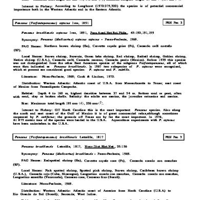
Click For Previous Page
May 2020 2
Motion For Cog Ownership
December 2019 15
Electrical Engineering Previous Paper-1998
June 2020 3More Documents from ""


Broadband Submission 2007
June 2020 7


